Worst Case vs Most Likely vs ALE

Author: Mike Yeomans. Manager, Cyber Risk Quantification

Summary: Worst case sets a practical limit on what should be spent to manage/mitigate risk, most likely is what you should expect to occur, while ALE tells you how to do long-term financial planning or to think for (self) insurance.

Clear communication is the key to effective risk assessment and management. By clearly communicating the results of a risk assessment, the assessor can enable decision-makers to know:

• What risks they have;
• How these can be managed;
• How this can be done in a cost-effective way.

While quantification based on data and the use of Monte Carlo methods improves analysis and provides better options for communicating risk, figuring out the best way to present results can still be tricky.

How should the results be presented to most clearly convey to stakeholders what your message is so that they know what they need to do?

The short answer is, it depends on what you’re trying to convey and who your audience is. When you’re trying to explain a concept or persuade someone to do something, there’s no point speaking a language that they don’t understand. That may mean presenting a full loss exceedance curve, the range of impact (e.g. 0-1m), operational equivalents (e.g. days offline), or more likely being asked to provide a point estimate such as the most likely, worst case, or the average loss expectancy (aka ALE)ⁱ.

When communicating the risk as a fixed integer, how can you know which to pick?

Useful for preparing for extreme (but possible) events.

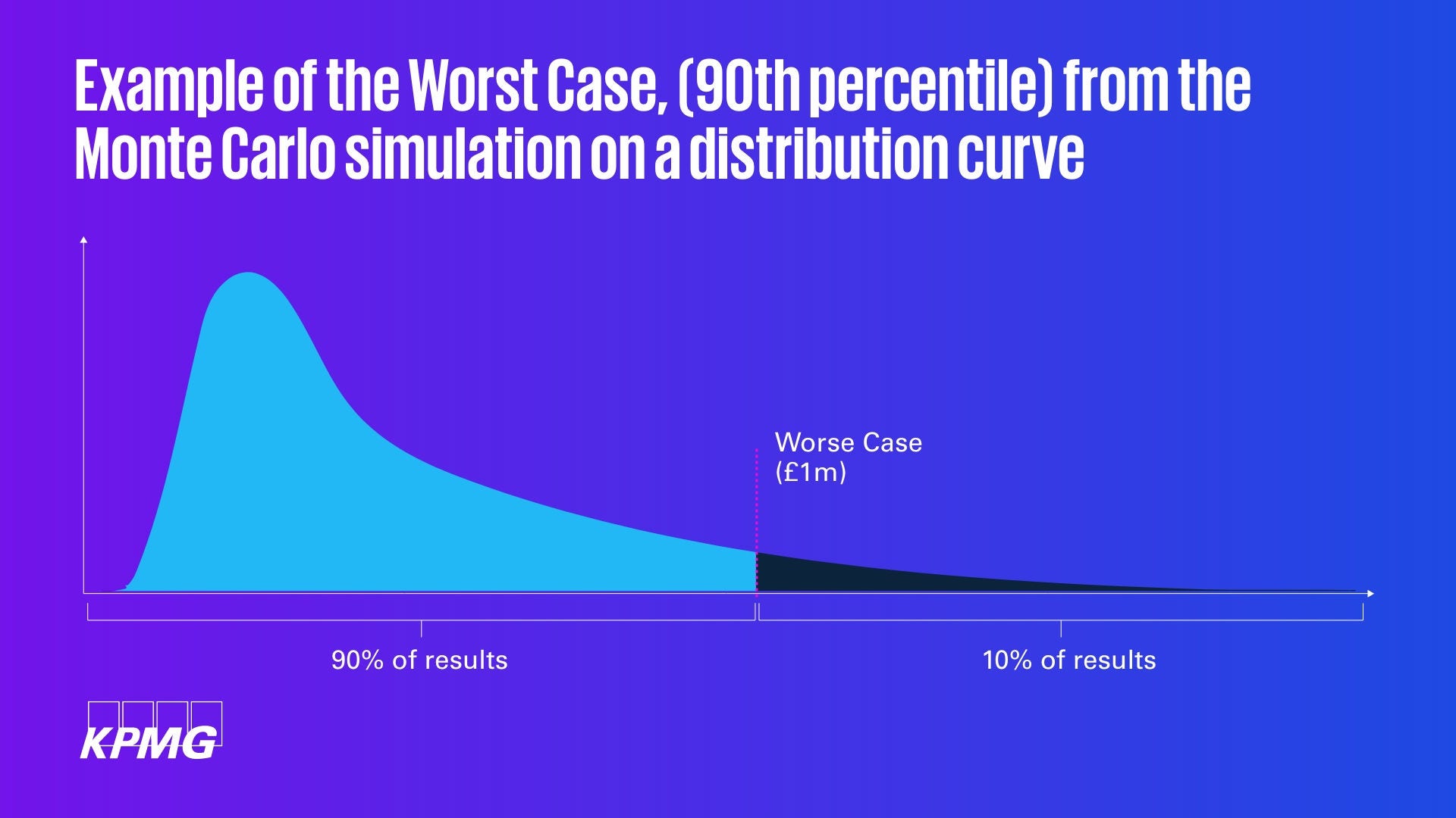
What: This one is largely self-explanatory. If the incident occurs, it will not have a more severe impact that the worst case. This is often the 90^th percentileⁱⁱ – i.e. a once in a decade (1/10) event (or some agreed tolerance level). The 90^th percentile indicates that 90% of all Monte Carlo simulation results come before this point (i.e. only 10% of results will have a greater impact than this figure). Different percentiles can be used to report the worst case based upon your individual worst case appetite (e.g. the 95^th percentile represents 1/20 or a 1 in 20 year event).

When: It often may not be helpful for conveying risk, but in contexts when planning is needed for catastrophic modelling, such as in financial capital requirements or for disasters and emergency planning (e.g. insurance, banking, or public sector planning).

Why: The worst case shows how severe a risk may be, setting the practical limit on how much should ever be spent to mitigate its potential (e.g. if cyber-attacks have a worst case risk of £1,000,000 of loss then it would wasteful to spend more than £1,000,000 to remediate themⁱⁱⁱ.

Limitation: The worst case value conveys an outcome that is highly implausible and will be of limited value to most decision-makers. It will be a large number that may prove distracting or potentially discredit the point if it gets latched onto (e.g. hijacks the conversation or gets you laughed out of the room – both of which have happened to me!).

Fig.1 Example of the Worst Case, (90^th percentile) from the Monte Carlo simulation on a distribution curve. As can be seen, in 9 out of 10 years (or 90% of simulations) witness losses less than £1,000,000. In 1 out of 10 year (1/10 or 10% of simulations) losses exceed this.

Perhaps the most helpful for reporting risk to leadership.

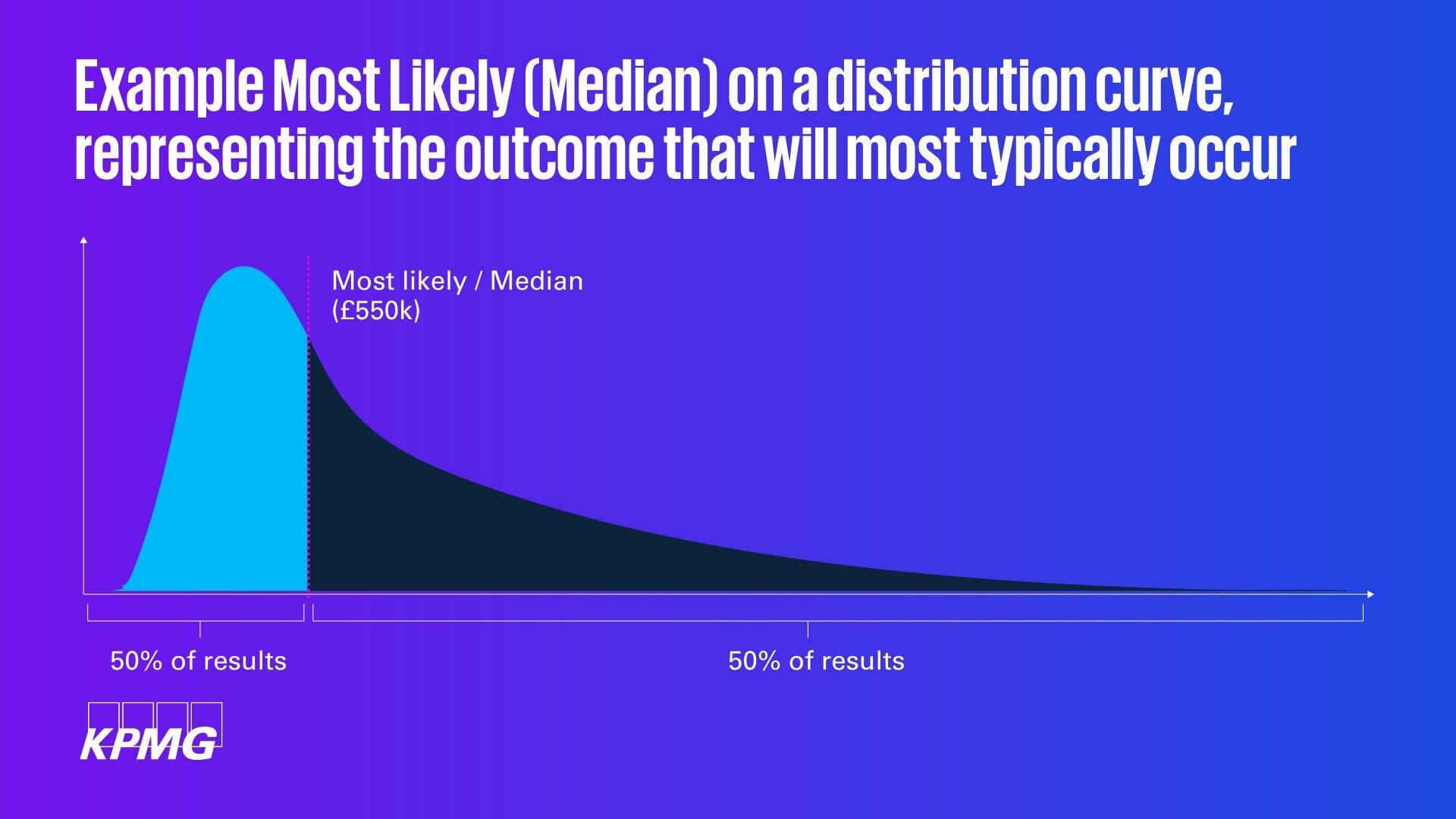
What: The Median figure of the Monte Carlo results, conveying the most likely amount of loss to be expected (i.e. if/when the risk materialises, this is what it will probably be)^iv.

When: The most likely is ideal for conveying risk to operational risk and security managers, as it gives them an understanding of what they need to prepare themselves for and how they should spend their annual budget.

Why: Most likely prepares you for the plausible and what is expected – essentially the cost of doing business and the amount you should spend to mitigate it (e.g. if accidental data disclosures will cost £20,000 per year, then an organisation should spend about £20,000 to mitigate the annual cost).

Limitation: The most likely figure advises decision-makers how to plan for day-to-day risk, but makes no allowances for more severe, less probable, but still possible outcomes. Strategic risk management cannot be optimally achieved if only managing for the most likely losses.

Fig.2 Example Most Likely (Median) on a distribution curve, representing the outcome that will most typically occur.

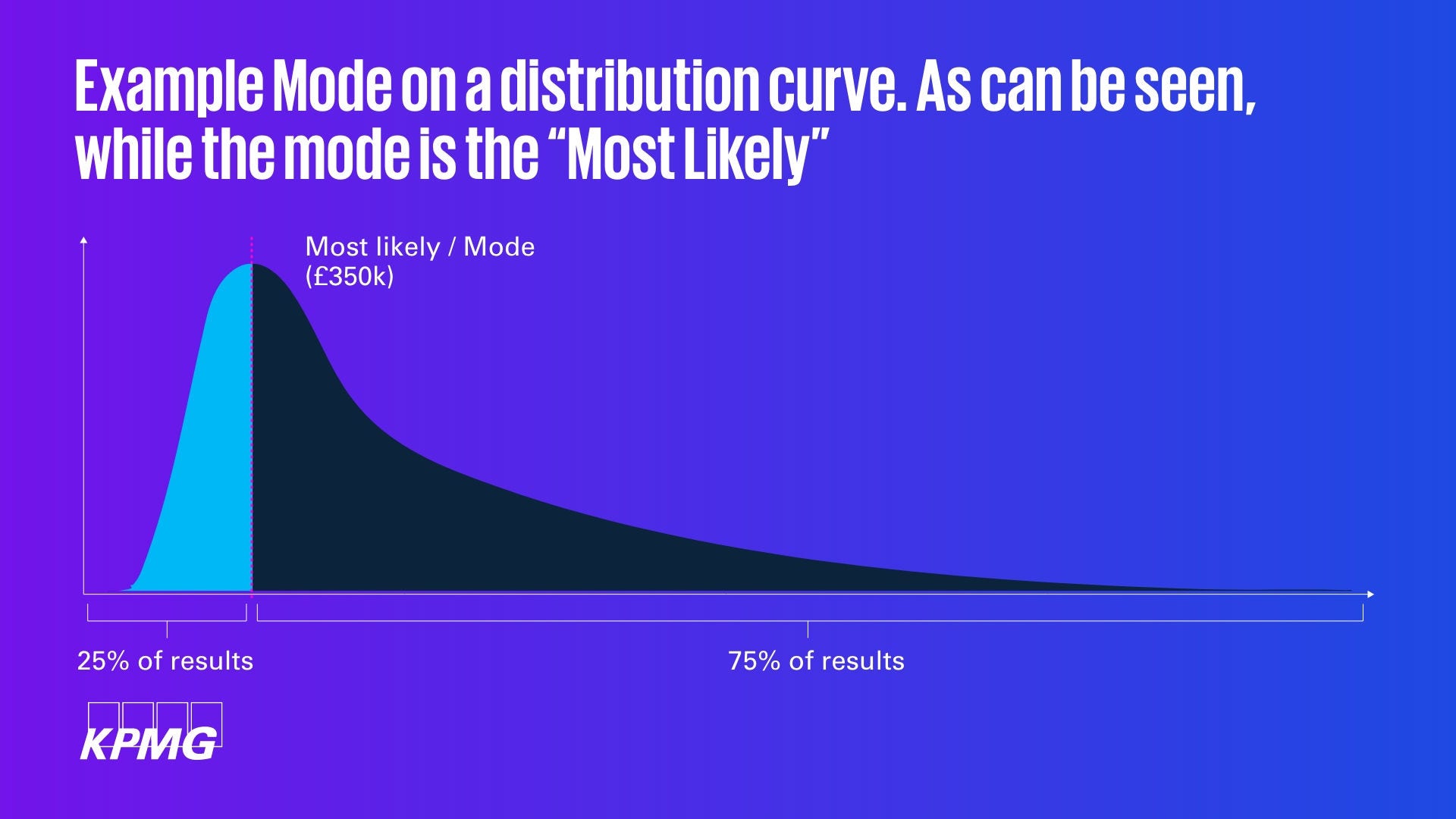
As noted, while the mode is the mathematical “true” most likely it problematic and potentially misleading to use. As can be seen from the graph below, the mode only represents a small proportion of simulated outcomes (significantly less than half), meaning it is not effective when planning/pricing for risk. This raises significant potential for leadership to lose confidence in your risk assessments, given actual losses will typically be greater than expected/forecast.

Fig.3 Example Mode on a distribution curve. As can be seen, while the mode is the “Most Likely”, it only occurs 25% of the time or less. In 3 out of 4 simulations (75% of the time) the losses are greater than the “Most Likely”

Additionally industries that rely on probability and forecasting for their revenue rely on being right just 50.1%+ of the time every time (or just above the median)^v. This further suggests that median is best to use when conveying the “Most Likely” figure.

Helpful for insurance.

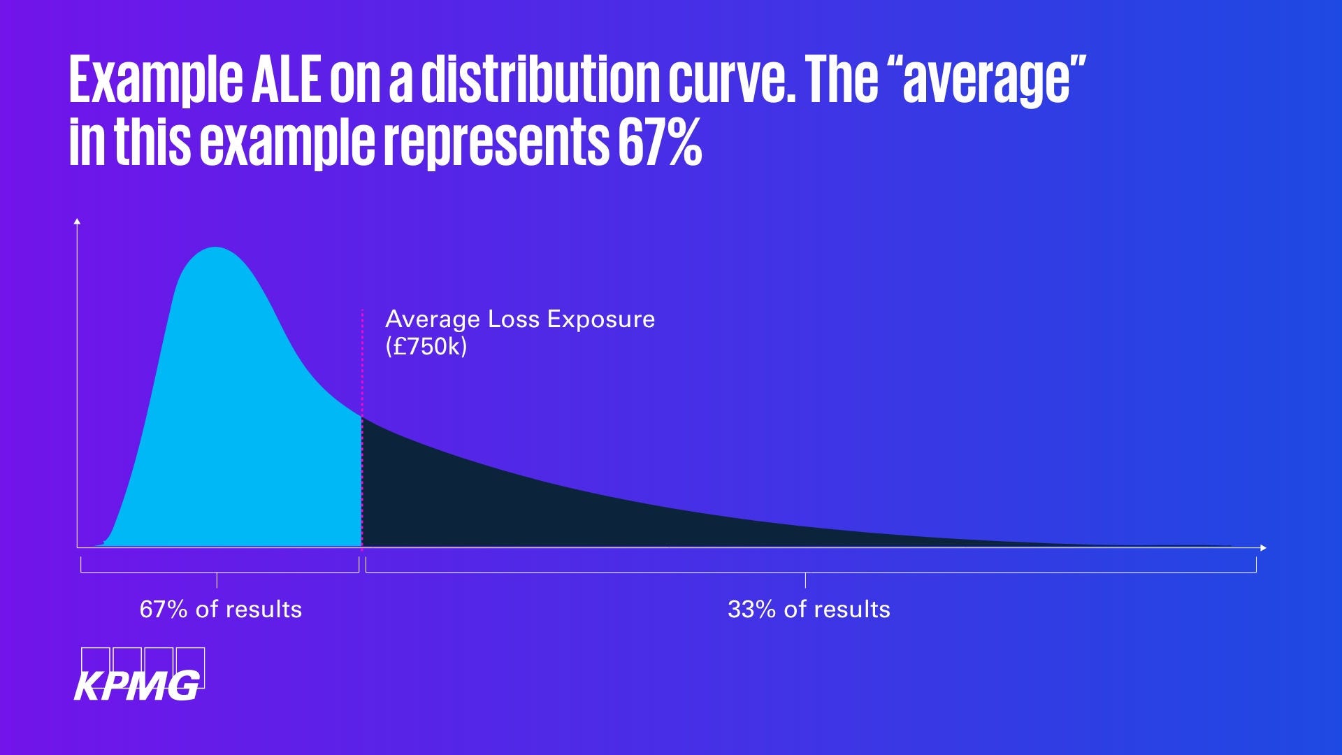
What: The ‘average’ (arithmetic mean) of the Monte Carlo simulation. It tells you the average loss that can be expected from an incident. While it can be pithy, simple to explain, and powerful, it also hides detail due to being somewhat simplistic^vi.

When: If decision-makers want a single figure to make strategic budgetary decisions around long-term financial planning (i.e. to self-insure against losses) then this is likely the figure for them. It is also used by insurers when pricing premiums, and can be used by organisations to have an approximate understanding for how much their premium should cost.

Why: ALE overestimates the typical or annual loss, but underestimates the worst case by a considerable way. To provide an example, if the annual most likely risk is £1, with a worst case of £10 (i.e. once a decade a loss of £10 will be incurred), then the ALE will be £2. This means that every year £2 will be saved. £1 will be lost due to risks incurred. But by the 10^th year, £10 will have been saved so that the organisation has the capital reserves to be able to incur a £10 loss (see table). This could be used either for self-insurance or (more plausibly) to determine what the level of investment in security mitigations that is cost-effective to take account of both the most likely and worst case scenarios.

Fig.4 Example of budgeting using ALE over a 10yr period

Limitation: It is not possible to know when the worst case (£10) loss will occur, meaning the investments may be insufficient to protect against a worst case risk if it were incurred in the near term. Likewise, as ALE is markedly larger than the most likely, the figure is unhelpful for day-to-day budgeting and may regarded as too high to be believable, making it difficult to justify the expenditure when trying to persuade decision-makers to increase cyber security budgets to plan for the long term.